Squaring the circle
This post is based on an undergraduate project which was done together with my colleagues:
Table of contents:
Mathematics is an active discipline! Whenever you see a question written in this style, I encourage that you attempt to solve it! Clicking the question will reveal the answer.
When someone tries to square the circle, it means that they are trying to accomplish a seemingly impossible feat. But what is this circle squaring all about, and is it really that difficult? In this blog post we’re going to explore this beautiful math problem that stumbled the ancient greeks, and we will show how the concept of field extensions provides a beautiful answer.
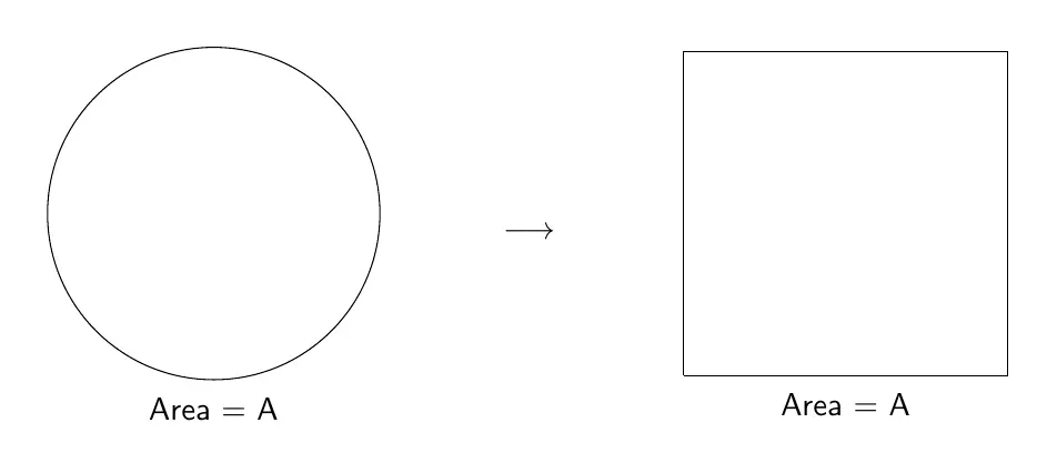
The problem
We start with a given circle of area \(A\), and the goal is to obtain a square with the same area \(A\).
But this should be easy! If the first circle has radius \(r\), then the area is \(A = \pi r^2\), and so we just need a square with side length \(l = \sqrt{\pi}r\), so that \(l^2 = A\), right? It turns out the problem is not so simple, as there are some rules on what lengths are we allowed to construct.
The rules
Ancient greeks wondered if one could obtain the desired square by only using ruler and compass. This means that, from a given set of points (in this case, the center of the circle and a point on the circle itself, so that their distance is the radius), we can only construct some of the remaining points in the plane (hopefully, the desired square vertices). So, what exactly are we allowed to do? Let’s suppose we start with just these two points in the plane:

One of the two points has been assigned the role of the origin point, and identified with \((0,0)\), and the other one serves as a way of defining a unit length, which is the distance between the two points. We then are allowed to perform the following operations:
- Ruler operation: Given two points, trace the straight line that passes through them.
- Compass operation: Given three points, \(P\), \(Q\) and \(R\), trace the circumference centered at \(P\) with radius the distance between \(Q\) and \(R\).
With these two operations, any intersection point of straight lines and/or circumferences we can trace becomes part of our working point collection. If we start with the two aforementioned points, what other points can we reach? Can we get the vertices of the desired square? We’ll dive into the answer step by step.
Building the constructible points
The first points that we can secure are those on the \(X\) axis that have an integer coordinate. That is, points of the form \((n,0)\) where \(n \in \mathbb{Z}\). All we need to do is trace the \(X\) axis by using our ruler with the starting points, and then, construct a circumference of unit radius centered at \((1,0)\). This circumference will produce \((2,0)\), and we can keep iterating this process to get every point:

As such, we obtain any integer distance \(z \in \mathbb{Z}\), between points \((0,0)\) and \((z,0)\). However, we still face two major problems: for the desired square, we’d want a non-integer distance to appear (remember, the side length needs to be \(l = \sqrt{\pi}r\)), and we’ve yet to obtain a point that’s not snapped to the X-axis. This second problem is actually easy to solve:

As you can see, by tracing a unit circle centered at \((0,0)\), and another at \((1,0)\), they intersect at two new points which don’t lie on the \(X\)-axis.
Notice that the three marked points in the previous figure form an equilateral triangle. Can you figure out the coordinates of our new point? What is its distance to the origin?
The points form a unit-sided equilateral triangle. Hence, the coordinates for the new point need to be \((\cos \frac{\pi}{3}, \sin \frac{\pi}{3}) = (\frac{1}{2}, \frac{\sqrt 3}{2})\). Another way of solving this is to realize that the point will have the form \((\frac{1}{2},y)\), since it lies in the perpendicular bisector of the segment formed by the other two, and then forcing the distance from this point to the origin to be \(1\). Obviously, this new point is at distance \(1\) from the origin, since it lies on the unit circumference centered at \((0,0)\).
“Parallelizing”
Our quest to reach the largest possible amount of points has to take a quick detour to gather the necessary tools that will allow the search to continue. We’re going to see how to obtain parallel and perpendicular lines. Firstly, given two points \(Q_1\) and \(Q_2\) that form a line \(l\), and a third point \(P\), we want the parallel to \(l\) through \(P\), that is, a second point \(P'\) such that the line connecting \(P\) and \(P'\) is parallel to \(l\). We start by tracing a circumference of radius \(\overline{Q_1Q_2}\) centered at \(P\):

Now, we trace a circumference of radius \(\overline{PQ_1}\) centered at \(Q_2\):

They intersect at \(P'\) with the desired properties!

Visually, it is clear that the new line is parallel to the previous one. Will this always be true?
Yes! Notice that, since \(P'\) lies on the circumference centered at \(P\) and with radius \(\overline{Q_1Q_2}\), then \(\overline{PP'} = \overline{Q_1Q_2}\). But also, since it lies on the circumference centered at \(Q_2\) with radius \(\overline{PQ_1}\), then \(\overline{PQ_1}\) = \(\overline{P'Q_2}\), so opposite side lenghts are equal and then \(P, P', Q_1, Q_2\) form a parallelogram, whose sides are parallel.
The perpendicular to \(l\) through \(P\) is actually very easy. We just need the typical construction of the perpendicular bisector:

If \(P\) doesn’t lie on the perpendicular bisector, then just use the previously explained parallel procedure to shift it!
The field of constructible numbers
So far, we’ve been talking about constructible points, which were those that could be obtained from the origin and the unit point. However, thanks to the results derived in the previous section, it doesn’t really matter if we consider points or numbers. For example if you can reach point \(P = (x,y)\), then you can obtain \(x\) itself (that is, the point \((x,0)\)) by tracing a parallel to the \(Y\) axis through \(P\) and letting it intersect the \(X\) axis.
Similarly, given points \(x\) and \(y\) which are constructible (again, this means one can obtain the points \((x,0)\) and \((y,0)\)), you can trace a circumference with radius \(y\) centered at the origin and let it intersect the \(Y\) axis to get \((0,y)\). With the appropriate usage of parallel lines, the point \((x,y)\) is then retrieved:

But wait! So far we had just constructed points in the \(X\) axis. It would be illegal to use the \(Y\) axis like we just did, since we didn’t get any point from said axis in the first place. Can you explain a way of constructing such a point, so that we can use it?
Since we already have the horizontal axis, and we know taking perpendiculars can be done, simply trace a perpendicular to the \(X\) axis through the origin. There are, of course, many other valid explanations.
This means that we can make our life easier by establishing the following definition: a number is constructible if and only if it’s any component of a constructible point (starting from \((0,0)\) and \((1,0)\)). We’ll denote this set of numbers as \(\mathcal C\). Constructible numbers and points are essentially the same, but it will be easier to work in one dimension. Note that \(\mathcal C \subset \mathbb R\), although we don’t know yet whether they are the same.
In order to use the powerful tools of algebra with our problem, we’re going to show some key properties of \(\mathcal C\). This set, along with the usual sum (\(+\)) and product (\(\cdot\)) operations, has a field structure. This means that certain operations are preserved. Let’s take a look at them with visual proofs.
Firstly, there are neutral elements for both operations, that is, elements such that, when summed or multiplied with another number, leave said number unmodified. They are, of course \(0\) (for the sum) and \(1\) (for the product), and them being constructible is the very first thing we established.
Secondly, the sum of constructible numbers is again constructible, and the same goes for the difference:

Same goes for the product. Here we show the construction, which cleverly uses Thales’s Theorem:

This same construction with a minor modification yields the multiplicative inverse:

With all these properties, as well as associativity and distributivity, which are automatically inherited from operations in \(\mathbb R\), we can conclude that \(\mathcal C\) is a field, as desired.
If you pay close attention to the last two figures, you’ll see that in order to apply Thales’s Theorem, we need the involved numbers to be positive (\(a,b > 0\)). Can you explain why multiplication and inverse work in general, even if the values are not both positive? You should be able to do this without any crazy construction, only with everything discussed so far.
Suppose, for example, that \(a < 0\) and \(b > 0\). Then, using Thales’s Theorem we can get \((-a)b\), but this is the same as \(-ab\). Then, you can do \(0 - (-ab) = ab\) to finish it off, since the case of the difference has already been proven in general. The case where both are negative is even easier, and the same goes for the inverse. Finally, if any of the numbers is \(0\), the product is \(0\) which is in \(\mathcal C\).
In previous sections we saw that every integer could be constructed, that is, \(\mathbb Z \subset \mathcal C\). It turns out that the smallest field that contains the integers is the rationals (can you see why with the properties discussed?), which automatically gives \(\mathbb Q \subset \mathcal C\). In other words, any point of rational coordinates can be constructed. That’s a lot!
Let’s wrap up this section with one last crucial property of \(\mathcal C\). Given the compass rule, it makes sense that if a point \((a,b)\) can be constructed, then so can its distance to the origin (the number \(\sqrt{a^2+b^2}\)). The way to do this is the obvious one (with a circumference centered at \((0,0)\) and intersecting the \(X\) axis). This allows non-rational numbers to be constructible: for example, \(\sqrt{2}\) is the distance of \((1,1)\) to the origin. It turns out that the square root of any positive, constructible number is also constructible, and the classical construction for this is the following:

Equipped with the knowledge that \(\mathcal C\) is a field where taking the square root is preserved, we are ready to prove that squaring the circle is impossible!
Algebraic field extensions
The key observation to prove the impossiblity of squaring the circle lies on algebraic field extensions. Suppose that, starting from \(\mathbb Q\), we have already constructed some of the constructible numbers \(\mathcal B \subset \mathcal C\). We can assume \(\mathcal B\) to be a field.
Why can we assume that \(\mathcal B\) is a field?
We know from the previous section that the constructible numbers, \(\mathcal C\), are a field. Hence, if we consider the smallest field containing \(\mathcal B\), that is, any number obtained from adding, subtracting, multiplying and inverting elements from \(\mathcal B\), this field has to consist only of constructible numbers, hence we can take this as our \(\mathcal B\).
Then, we further construct another point \(P = (x_0,y_0)\), hence reaching both \(x_0\) and \(y_0\). How do these two values relate to those in \(\mathcal B\)? It actually depends on how they’re constructed.
First case. If they were obtained intersecting two lines through points in \(\mathcal B\), since these lines have equations \(ax+by = c\) and \(dx+ey=f\), with \(a,b,c,d,e,f \in \mathcal B\) (you can check this by explicitly taking two points with coordinates in \(\mathcal B\), writing the line equation, and using that \(\mathcal B\) is a field), it follows that their intersection is: \((x_0,y_0) = (\frac{ce-fb}{ae-bd}, \frac{af-cd}{ae-bd})\). Since \(\mathcal B\) was a field, then actually \(x_0,y_0 \in \mathcal B\) so we didn’t construct anything new.
Second case. If they were obtained intersecting the line \(ax+by=c\) and the circle \((x-d)^2+(y-e)^2 = f^2\), where once again \(a,b,c,d,e,f \in \mathcal B\), we can compute the intersection similarly. For example, if \(b \neq 0\), we write \(y = \frac{c-ax}{b}\) and this gives that \((x_0-d)^2 +(\frac{c-ax_0}{b}-e)^2 = f^2\). This is, \(x_0\) satisfies a polynomial equation of degree \(2\), whose coefficients are in \(\mathcal B\). In other words, \(x_0\) is the root for a degree \(2\) polynomial in \(\mathcal B\). The same goes for \(y_0\) in the event that \(a \neq 0\).
What relation do we obtain if \(b = 0\) (similarly for \(a=0\))?
In this case, simply looking at the line yields \(x_0 = \frac{c}{a}\) so \(x_0 \in \mathcal B\).
Third case. As you might have already guessed, the third case involves intersecting two circles:
\[(x-a)^2+(y-b)^2 = c^2\]and
\[(x-d)^2+(y-e)^2 = f^2,\]with \(a,b,c,d,e,f \in \mathcal B\). One can subtract the two equations to obtain a new equation
\[2(a-d)x + 2(b-e)y = f^2-c^2+a^2+b^2-d^2-e^2,\]which is that of a line, and intersecting this line with any of the two circles gives the point \(P\), so we’re back to case \(2\).
The key thing we’ve checked is that if the new element wasn’t already in \(\mathcal B\), then it satisfies a degree \(2\) polynomial with coefficients in \(\mathcal B\). In mathematical terms, this means that the new element is algebraic over the field \(\mathcal B\). If we denote by \(\mathcal B (x_0,y_0)\) the new field that arises upon adding the new points (and building a field as explained before, by adding, subtracting, multiplying and inverting the elements), this means that \(\mathcal B (x_0,y_0)\) is an algebraic extension of the field \(\mathcal B\) (because it was obtained by adding algebraic elements). A result from field theory establishes that every element of an algebraic field extension is algebraic (not only the ones we manually added), but we won’t need this for our argument.
Towering extensions
Let’s imagine how the previous section fits into our construction process. We first obtained that \(\mathbb Q\) was constructible. Now we further construct another point \(P_0 = (x_0,y_0)\), which gives us an extension \(\mathbb Q \subset \mathbb Q(x_0,y_0)\) which is algebraic, so that \(x_0\) and \(y_0\) both satisfy a polynomial with coefficients in \(\mathbb Q\) (whose degree is at most \(2\)). Now, from these points, we further construct \(P_1 = (x_1,y_1)\). The previous analysis tells us that \(x_1\) and \(y_1\) will satisfy a polynomial with coefficients in \(\mathbb Q(x_0,y_0)\). In other words, we have the following extension tower: \(\mathbb Q \subset \mathbb Q(x_0,y_0) \subset \mathbb Q(x_0,y_0,x_1,y_1)\), where any pair of consecutive extensions is algebraic. For these situations, there is a key result from field theory:
Theorem 1. If \(K \subset L \subset M\) is a tower of field extensions, where every two consecutive extensions are algebraic, then \(K \subset M\) is also algebraic. In other words, if elements in \(L\) satisfy polynomial equations with coefficients in \(K\), and elements in \(M\) satisfy polynomial equations with coefficients in \(L\), then elements in \(M\) will satisfy a polynomial equation with coefficients in \(K\).
The proof needs a decent amount of theory that doesn’t fit here.
Theorem 2. Any constructible number \(c \in \mathcal C\) satisfies a polynomial equation with coefficients in \(\mathbb Q\).
Let’s recap why:
- We started from \(0\) and \(1\) and constructed the whole of \(\mathbb Q\) by realizing that the constructible numbers are a field.
- We construct a new point \(P_0 = (x_0,y_0)\), which gives a whole new field of constructible elements, \(\mathbb Q(x_0,y_0)\), and \(x_0\) and \(y_0\) satisfy polynomial equations with coefficients in \(\mathbb Q\).
- On each step, we construct a new point \(P_i = (x_i,y_i)\) which gives a new field, and \(x_i\), \(y_i\) satisfy polynomial equations with coefficients in the previous field. By Theorem 1, this means that \(x_i\) and \(y_i\) actually satisfy equations with coefficients in \(\mathbb Q\), as desired.
The final proof
Theorem 3. It is impossible to square the circle. That is, starting from a circle which can be assumed centered at \((0,0)\) and of unit radius, it is impossible to obtain, using ruler and compass, (the vertices of) a square with the same area \((A = \pi)\).
Proof. Since we start from the circle centered at \((0,0)\) and of unit radius, this can be rephrased as starting from \((0,0)\) and \((1,0)\) as we’ve been doing. If squaring the circle were possible, the side lengths of the square would also be constructible (why?). This would imply that \(\sqrt{\pi} \in \mathcal C\), and, in turn, that \(\pi \in \mathcal C\). However, \(\pi\) is a transcendental number, that is, it cannot satisfy a polynomial with coefficients in \(\mathbb Q\), contradicting Theorem 2. \(\tag*{$\blacksquare$}\)
The fact that \(\pi\) is transcendental is not easy to show, and can be deduced from a theorem due to Lindemann and Weierstrass.
Parting words
Congratulations for making it here! This was quite a dense post, but I hope you could learn something along the way! There are other marvelous results that can be proven using all this theory, which closely relates to Galois Theory. Here I leave you some more questions that will allow you to further explore this topic if you want to.
Observe Theorem 1 carefully. There’s a relationship between the degrees of the polynomials involved. Suppose we have a tower of the kind \(\mathbb Q \subset \mathbb Q(x_0) \subset \mathbb Q(x_0, x_1)\), as before. If \(x_0\) satisfies a polynomial of degree \(d_1\) with coefficients in \(\mathbb Q\), and \(x_1\) satisfies a polynomial of degree \(d_2\) with coefficients in \(\mathbb Q(x_0)\), then the degree of the polynomial satisfied by \(x_1\) with coefficients in \(\mathbb Q\) (as per Theorem 1) turns out to be \(d_1 \cdot d_2\). Using this, given a constructible number \(c \in \mathcal C\), what can you say about the degree of the polynomial in \(\mathbb Q\) it satisfies?
Since, from every field to the next one, a polynomial of degree \(1\) or \(2\) was involved, using the previous question we deduce that the degree has to be a power of \(2\). For example, \(2\) or \(4\) would be obtained with this procedure, but not \(3\).
Is it possible that \(c \in \mathcal C\) satisfies a polynomial with a different degree from the one obtained in the previous question?
Yes, because if \(P(c) = 0\), then \(c^kP(c) = 0\) for any \(k \in \mathbb N\), so you could obtain any degree which is greater than the one obtained in the previous question via considering the polynomial \(X^kP(X)\).
Theorem 4. If we restrict every polynomial discussed so far to be irreducible, then the answer to the previous question is no. In other words, if \(c \in \mathcal C\) is constructible, and \(P(X)\) is an irreducible polynomial with coefficients in \(\mathbb Q\) so that \(P(c) = 0\), its degree is necessarily the one obtained in the first question of this section.
(Hard question) Use these facts to show that it is impossible to duplicate a cube with ruler and compass. That is, given a cube with two of its adjacent vertices at \((0,0)\) and \((1,0)\), it is impossible to construct (the vertices of) a cube with double the volume (that is, volume \(V = 2\)). Use the results from this section, as well as the proof for the circle squaring impossibility.
If you got it, congrats! Contact me if you want to discuss this question.
(Extra hard question) Use these facts to show that it is impossible to trisect the 60º angle with ruler and compass. That is, given the points \((0,0), (1,0)\) and \((\frac{1}{2}, \frac{\sqrt{3}}{2})\), which form a 60º angle, it is impossible to construct the point \((\cos \frac{\pi}{9}, \sin \frac{\pi}{9})\), which would correspond to a third of the angle. Use the results from this section.
If you got it, congrats! Contact me if you want to discuss this question.